|
| Output of new Market area coverage by distribution facilities |
This weeks lab involved using Location Allocation solver in ArcMap. Location allocation can be used to determine where to place a new store, fire station, or, in the project performed here, service area of a distribution center. We were provided with an original market area map showing which distribution centers serviced which market areas. The key is that the original distribution center service areas were generated organically, over-time. Thus the true nature of our analysis was to determine which service areas should be changed. The output from the location allocation analysis (see right) shows that several areas (13 total) were better served by a different distribution facility than the one originally selected for it. Overall, location allocation solver in ArcMap is a fundamental tool in large-scale data analysis, otherwise not logistically possible.


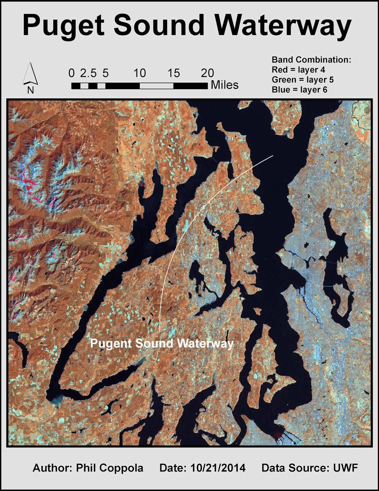 This weeks lab involved using multispectral analyses processes to locate specific features within aerial imagery. Generally four steps are followed: 1) examine histograms of the imagery pixel data; 2) visually examine grey scale image; 3) visually examine multispectral image; 4) use inquire cursor tool to isolate specific cell values. The following are three such examples of this process. Features are highlighted by their contrast to background features.