Module 10 Lab: Supervised Classification

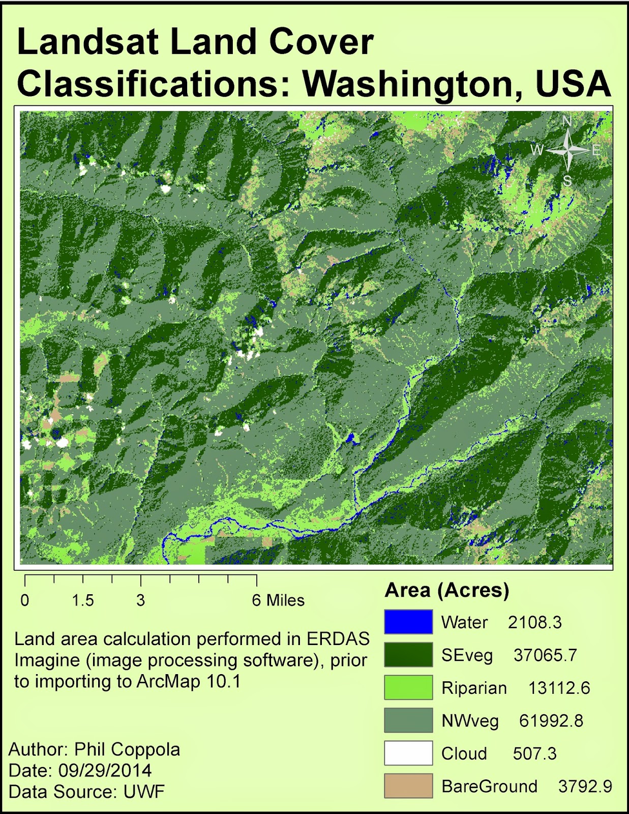
Above is a supervised classification of Germantown, Maryland generated using
ERDAS Imagine supervised classification.  The map was ultimate composed in
ArcMap.

1.      I used the seed polygon method to generate the signature polygons.  A distance threshold value of approximately 25-50 was generally used.  In cases when only one class was created and the class was relatively obvious, for example water, then I used a higher distance threshold value.  In cases when there were many classes for the same classification, for example Agriculture 1-4, I used a lower threshold values.  The lower values and many classes allowed for high coverage with minimal (or none) mis-classification.

Module 9 Lab: Unsupervised Classification

A map depicting the unsupervised classification of University
of West Florida campus.  There are four different Information
Classes.

Module 8 Lab: Thermal & Multispectral Analysis

Multispectral image of Coastal Ecuador highlighting the
color contrast of several distinct features.

The portion of the map that I selected is an agricultural area of the river bank.  I chose this entire area because it was a diverse area, thus providing a good contrast of land features.  There is a freshwater river with a forested island, and on the main land is an agricultural area surrounded by an urban area.  The band combination that was selected appropriately highlights these different features.  Red was linked to Layer 4, Green was linked to Layer 2, and Blue was linked to layer 6 (Thermal IR).  Accordingly, the vegetated island (high NIR, low temp) appear bright red, the urban areas to the east (low NIR, high temp) appear bright blue, and the main river (low NIR, low temp) appears green.

         Further, shape and pattern are useful in identifying these features.  Agricultural lands are often regular polygons (rectangles, or otherwise straight-edged) and would be expected to appear more blue than red in my image, which is the case.  The river and forested island are obvious based on association.

Module 7 Lab: Multispectral Analysis

 This weeks lab involved using multispectral analyses processes to locate specific features within aerial imagery. Generally four steps are followed: 1) examine histograms of the imagery pixel data; 2) visually examine grey scale image; 3) visually examine multispectral image; 4) use inquire cursor tool to isolate specific cell values. The following are three such examples of this process.  Features are highlighted by their contrast to background features.

Module 6 Lab: Spatial Enhancement

Image Enhancement output from ERDAS Imagine and ArcMap
Processing. 

This week's lab involved image enhancement using ERDAS imagine and ArcMap processing tools.  Raw aerial imagery often requires processing steps to produce an image that is spatially and radio-metrically correct.  Image processing software often performs automated enhancement to such images. ERDAS imagine and ArcMap were used to process an image (output seen at right).

Module 5a Lab: Intro to ERDAS Imagine and Digital Data 1

Final map output of landcover generated from
Landsat data first processed in ERDAS Imagine
and ultimately in ArcMap.

This week's lab introduced ERDAS Imagine image analysis software.  This software may be used to aid in the classification of land cover, as well as various other digital image processes and analyses.  We imported land cover raster data sets, manipulated and processed them in Imagine, and ultimately generated a final map output using ArcMap (see map to right).

Module 4: Ground Truthing and Accuracy Assessment

A map depicting accuracy proofing of LULC data of Pascagoula, MS. 

This lab involved truthing a Land Use Land Cover (LULC) classification map which was generated last week.  Ground truthing was done ex situ using Google StreetView of the area.  Much of the area was inaccessible from StreetView (western marshes) and were truthed using high resolution aerial imagery.

The overall accuracy is determined by comparing random points placed on the original LULC map to those same points found in Google StreetView or aerial imagery.  The overall accuracy of the LULC is determined by the number of "true" points divided by the total points.  The accuracy of my LULC map was 77%.

Module 2 Lab: Visual Interpretation of Aerial Images

This was my first module for Remote Sensing and Photo Interpretation course.  The focus of this lab was on identifying features within aerial images.  The first exercise involved locating areas of an aerial image that displayed different tones.  Tones, or brightness, may help the user identify features at those locations.  Next, texture, another good diagnostic tool for feature identification was exemplified.

In the second exercise, specific features were identified using size and shape, patterns, associations, and shadows.  Once a single object is positively identified (with a high degree of certainty) than it can be used as a reference in identifying other features.  For example, once you locate and identify a road, you can confirm the identity of a vehicle.  Then a building can be identied.  Because these aerial images have no scale to reference, within-image references are very useful.  A knowledge of the area (Pensacola BEach in map 2 at right) allows the user to determine water and pier features.