Showing posts with label GIS5103. Show all posts

Tuesday, August 5, 2014

Module 11: Sharing Tools

This week's assignment involved properly packaging and sharing a tool.  This required setting correct parameters, relative file extensions, and providing metadata.  The tool generated an array of random points placed within a specified area, then created a buffer around each point (screenshot at right).  The Description for the tool was edited in ArcCatalog so that it was more user friendly, providing easy-to-follow parameter requirements.  The script from which the tool was based was then directly embedded into the tool and password protected.  Embedding the script in this way reduces the number of individual files that must be sent to another user for the tool to run properly, and it provides security (using password protection) against unwanted interceptors of the tool's script.

As this is our last module, below is a recap of the GIS Programming Course...
Employing the existing capabilities of a GIS, Python scripting can be used to complete otherwise time-intensive geoprocessing tasks.  This GIS Programming course provided a solid foundation for future work within the field.  We started with an introduction to pseudocode, a near-English version of a script that provides a workable rough draft for the author and a potential reference to another user.  We then explored similarities and differences between Python scripting and ModelBuilder in ArcMap.  Next, were several modules that involved writing and editing Python scripts to perform various tasks and produce desired outputs.   During these weeks, a level of comfort in working with Python was achieved.  Both raster and vector datasets were manipulated and scripting proficiency was quickly increasing.  Debugging and error checking procedures were followed in PythonWin so that script issues could be quickly discovered and fixed.  Finally, custom tools were created and shared.  Python is a fundamental tool in the GIS professional’s tool belt as it allows for complex analysis and timely output production.  This course was broad and deep in content and thorough in delivery – a great experience overall.

Friday, August 1, 2014

Module 10: Creating Custom Tools

Custom Tool window
Script Message output
 This week's assignment involved creating a new geoprocessing tool in ArcMap using Python scripting.  Creating custom tools is an important aspect of GIS Programming because time-intensive geoprocessing operations may be completed in a quick, automated manner.  The general steps of creating a custom tool are as follows:
1.       Generate a script that contains unspecified input and output variables and will complete a process of interest
2.       Create a new toolbox in ArcMap using the Add > Toolbox dropdown in ArcCatalog
3.       Add the script (the script generated in step 1) to the toolbox
4.       Set the parameter options for the script/tool
5.       Connect the input parameters of the tool to the input and output variables in the script
6.       Add messages to check for progress of the tool and for debugging issues.

7.       Check to see if output is as desired, if not then debug script

Friday, July 25, 2014

Participation Assignment #2: Migration Patterns of Northern Saw-Whet Owls

 Beckett, Sean R. and Glen A. Proudfoot. 2011. Large-scale Movement and Migration of Northen Saw-Whet Owls in Eastern North America.  The Wilson Journal of Ornithology 123(3):521-535.
In this paper, researchers mine a bird banding database to tease apart patterns of migration and large scale movement for the Northern Saw-whet Owl (NSWO) in eastern North America.  The United States Geological Survey (USGS) oversees several bird banding stations in the United States and manages the large database produced from them.  Bird banding stations are permanent, semi-permanent, or temporary field locations where ornithologists capture target bird species and place on them leg bands engraved with unique serial numbers.  The overall number of birds caught at specific banding stations may fluctuate seasonally or annually; thus, population trends or mass movement patterns may be detected using relevant spatiotemporal analyses.  Further, birds with bands can be recaptured within or between years so that individual movement and migration routes can be analyzed.
The Northern Saw-Whet Owl is a small owl that resides in the United States.  This study attempts to use banding records of this bird to determine if it migrates southward during the fall season, if individuals follow similar migration routes between years, and whether there is any age-related differences in movement.  They use a GIS (ArcView 9.3; ESRI 2008) to complete these analyses.
They examine the number of banded NSWOs using of 01° latitudinal lines as groups.  They find that the peak banding day – i.e. the mean Julian day – occurs later in the year as your move further south.  Thus they determined that NSWOs have a mass migration south during the fall months (fig. 3, Beckett & Proudfoot 2011).  Then, by creating vectors from original owl capture to recapture locations, they generated a rose diagram depicting the southerly movement for the birds during fall (fig. 5, Beckett & Proudfoot 2011).
This paper is significant in that it answers a large-scale question utilizing a public-access database – in other words the data was gathered, not collect, by the researchers.  They illustrate the use of databases and GISs as a foundational tool for understanding ecology of animal populations.  With increasing technological advances and utilization, similar research will continue to be produced.

link to paper: http://www.projectowlnet.org/wp-content/uploads/2011/09/Beckett-and-Proudfoot-2011-Wilson.pdf

Thursday, July 24, 2014

Module 9: Debugging & Error Handling

Output for Script 1

Output for Script 2
Output for Script 3
This weeks lab involved debugging and error handling, perhaps the most frustrating part of writing scripts in Python.  There are three types of errors encounter in Python: syntax errors, exceptions, and logic errors.  They can arise from improper character entry into the program, or from errors in geoprocessing.

The assignment involved debugging three scripts in various ways, creating the outputs seen at right.  PythonWin contains its own debugging interface, which was used to help the user locate or trap exceptions.  In the Output for Script 3 (below), an error message is presented, but the script was allowed to continue. Essentially, that portion/block of script was passed over.

Friday, July 18, 2014

Module 8: Working with Rasters

Final raster output that meets all criteria.
This week's lab involved working with rasters using the spatial analyst module in arcpy package.  Rasters allow for the display of continuous spatial phenomena and analysis using a GIS has made complex processes relatively simple.  The final lab output was a raster meeting three specific criteria.  These were: a specific landcover type, a slope between 5 - 20 degrees, and an aspect between 150 - 270 degrees.  The script written uses only DEM and landcover inputs.  At rights is a final raster output, below is a discussion of an issue that I encountered during the lab and how it was resolved.

1.     The only issue I had was that my final map displayed a raster with values of 1, 0, and NoData and thus looked different than the example shown on the assignment PDF.  Immediately I recognized that this was likely due to the landcover reclassification step.  The original script was as follows:

>>> outreclass = Reclassify("landcover", "VALUE", myremap, “NoData”)

2.       I investigated the Reclassify tool’s syntax through ArcMap help > Reclassify tool.
3.       “NoData” was displaying differently because I had specified it to do so in the script.  The final argument of how to represent NoData was optional, but I had entered it in.  The original script was copied from the Mod8 Exercise, this was the root of the problem.  In the Mod8 Exercise we purposely wanted to specify cells with NoData; however, in the Mod8 Assignment, we want to specify all cells that do not meet the criteria with a value of 0.
4.       Therefore, I removed the last, optional argument in the original script, creating the following final script, which ultimately produced the correct final raster:


>>> outreclass = Reclassify("landcover", "VALUE", myremap)

Friday, July 11, 2014

Module 7: Working with Geometries

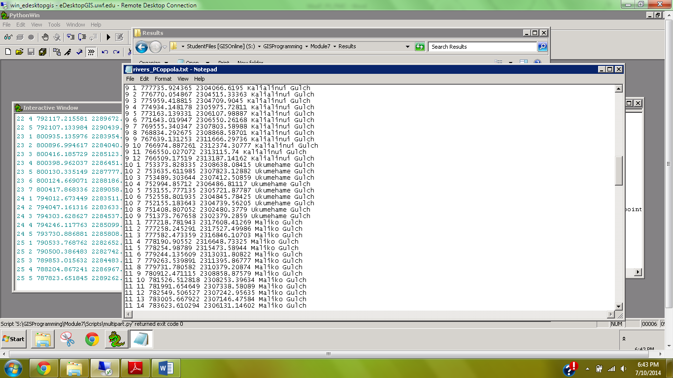
Screenshot of rivers_PCoppola.txt file
This week's lab focused on the conceptual and tangible connection between geometric/vector objects and the attribute table.  Specifically, we worked with features, arrays, and vertices by using cursors and tokens to produce a .txt file of select items from the attribute table (see screenshot at right).  The feature was a system of rivers (polyline feature class) on Hawaii.  We wrote a script that would iterate through all the arrays of this feature class and provide an output of the feature number, vertex number, x,y-coordinates, and feature name.  This required nested for loops to iterate over the embedded arrays.

Friday, June 27, 2014

Module 6: Exploring & Manipulating Spatial Data

Python Script Output
This weeks assignment was to dive deeper into Python scripting by manipulating lists, dictionaries, tuples, and using cursors.  List, dictionaries, and tuples are similar in that they store indexed data, however there are nuances to each that allow for diverse usage.  Spatial data is often stored in some sort of indexed format (tables) which must be easy to reference and manipulate.  The assignment here involved generating a geodatabase and editing some fields of a feature class within.

At right is a screenshot of my script output, which was used to select only county seats from a list of cities and then match each county seat with its population using a dictionary.  Below is a discussion of some issues I had during write-up and how they were overcome.

I had the most trouble with Step 5, which involved setting the search cursor to retrieve three fields while using an SQL query to only select County Seat features.  The issues occurred in three places of this step:  1) Setting the workspace; 2) calling the correct feature class; and 3) determining the syntax of the Search Cursor.

The first issue was merely an unnoticed typo, but it cause a lot of troubleshooting because I thought other parts of this step were causing the error message.  Typos are small errors that can cause big headaches.  Once realized this, it was quickly fixed and I moved on.

The second issue was a result of not knowing what file extension to use for the feature class cities in the new geodatabase.  I first used .shp, but this gave me an error saying that the file could not be located.  I then used windows explorer to determine if the extension had changed, and I found that it had changed to .spx.  Therefore I tried calling the feature class using this extension.   This again gave me the same error message.  I then thought that perhaps the basename extraction step (i.e. removal of .shp during copying step), produced a file with no extension, therefore I tried simply using ‘cities’, and this worked.  I then moved on to issue three.


Issue three was the toughest because I wasn't sure whether to use brackets, parentheses, quotation marks, commas, semicolons, etc. when using the Search Cursor.  Essentially the amount of info that was covered this week left me a little confused.  I realized, however, that I was over-thinking the problem.  I knew that the three fields needed to be within brackets, separated by commas, and within quotes.  Then I referred back to the exercise to determine how to use the SQL query, which was straightforward.

Monday, June 23, 2014

Week 6: Visibility Analysis

Finish Line Camera Coverage Map (symbology described in text)
This weeks lab involved using Visibility analyses on topographic data.  Specifically, we utilized Line of Sight, Visibility, and Viewshed tools (among others) in the 3D Analyst toolbox.  We worked with DEMs to determine what regions were visible from both point and line features and compared the outputs of these tools.

We also used veiwshed analysis to make an informed decisions about surveillance camera placement around the finish line of the Boston Marathon.  We were restricted to a 90 degree field of view for our cameras, and there were several buildings which obstructed possible placement.  I first analyzed aerial imagery to determine building locations, as I wanted to place the cameras on top of a tall structure.  I then used a DEM which included building height to determine how high these cameras would be placed.  The viewshed tool produced a raster with cell values from 0 - 3, where the value represented the number of cameras that captured that particular cell.  Cells with a value of 3 were colored red, 2 were yellow, and 1 were green (zeros were omitted).  Above is my output using this symbology.  [The cameras are magenta triangles and the finish line a blue dot].  All three of the cameras had an unobstructed view of the finish line as well as much of the surrounding area.

Friday, June 20, 2014

Module 5: Geoprocessing Using Python

This weeks assignment was to become familiar with geoprocessing in Python.  This was primarily accomplished by writing scripts that performed sequential geoprocessing tools in the arcpy site package.  The following is a breif transcript of my notes to complete the assignment.
1. First, I looked in the help window for a description on the Add XY tool as well as the Dissolve tool, just to get an idea of how they worked and what they did.
2. Next, I opened the ArcMap Interactive Python window as well as the PythonWin program.  I first used the scripts in ArcMap so that I could visually see what was happening to the data, then copied the text to a new script file in PythonWin.
3. Because the script should be standalone (outside of Arcmap), it first required to import the arcpy site package.  Then, I imported environment class and set the overwrite option to ‘true’.
4. Then I used the three tools in sequence: Add XY, buffer, and dissolve.  I followed the syntax described in the help folder as well as the easy to follow interactive python help window in ArcMap.
5. After each tool I added the GetMessage function.  Further I used the  ‘+ “\n”’ after the first two tools so that the message was easier to read.
6. I tested the tool in PythonWin and ArcMap to see if the desired result occurred; it did.

Friday, June 13, 2014

Module 4: Python Fundamentals - Part 2

This weeks assignment involved debugging an existing script as well as writing our own to produce a desired outcome.  A script that was given to us was supposed to produce a simple dice rolling game between several participants, but it had several errors in need of correction.  To fix these errors, the debugging toolbar was used and error messages were interpreted.  Eventually the output was produces as seen above.

We were then required to randomly generate a list of 20 integers between 0-10 and remove a specific 'unlucky' number.  I chose the number 6 as my “unlucky” number, which was removed.  To print the number of times that 6 appeared in my original list, I used the if-elif-else structure.  Using the count method to determine the number of 6’s in the list, I chose the following three conditional outputs:

If there were no sixes, then it would print “This list contains no sixes.”  If there was one six, then it would print “This list contains 1 six, which was removed.”  If there were multiple sixes, then it would print “This list contains (the number of sixes), which were removed.  
I used the while loop and the remove method to remove each six sequentially from the list until the list contained no sixes.  Then the new list with all sixes removed would be printed.

Friday, June 6, 2014

Module 3: Python Fundamentals - Part 1

This week's assignment was to become familiar with Python scripting language.  We used Python to perform a few basic functions and methods.  We were instructed to start with a string object of our full name and write a script that ultimately printed only our last name and the number of letters in our last name multiplied by three.  The output of my script is seen above.

This was multi-step process in which we had to isolate each name in a list (e.g. first, middle, last), select only our last name, then calculate the number of letters in it.  This was achieved as follows:

1.       I used my full name “Philip Michael Coppola” as the original string and split this string into a list, which I called “listName” indexed as 0 (Philip), 1 (Michael), 2 (Coppola).
2.       I then used the script:
>>>lastNameLen = len(listName[-1])
>>>print lastNameLen

This gave a result of ‘7’, the length of “Coppola”.  Due to the requirement that another person should be able to use this code to print their last name, I had to use the [-1] index.  This references the last item in a list, whereas using [2] would only work if the other person put three names.

Thursday, May 29, 2014

Participation Assignment 1: GIS-based Red-cockaded Woodpecker Foraging Matrix Application

               
Red-cockaded woodpecker
(Photo Credit: USFWS)
 The red-cockaded woodpecker (RCW) is a federally endangered bird endemic to the United States.  It has been at the forefront of conservation efforts due to its dramatic decline in recent decades.  RCWs are obligate residents of old growth pine forests of the Southeast United States, an ecosystem that is highly fire-dependent.  The United States Fish and Wildlife Service (USFWS), the government agency responsible for harboring and protecting endangered species, has created a GIS-based habitat index matrix which scores suitable foraging habitat in the vicinity of know RCW recruitment locations.
                RCWs roost and nest in excavated cavities of living pine trees which are arranged in small clusters, with one bird per cavity.  Thus they have a “home” cluster to which they return each night after spending the day foraging and that they fiercely defend from adjacent RCW families.  Their foraging efforts are most efficient if they utilize habitat within a specific radius of their home cluster.  The RCW foraging matrix is used to quantitatively score the habitat within such a radius of a cluster.  The analysis is based on the assumption that RCW families will primarily forage within this area.
Array of cluster locations and circular buffer with
overlaid land use data
(Photo Credit: USFWS)
Concentric rings of varying radii from an RCW cluster are analyzed for suitability.  Forestry and land use data (dominant tree type, stand density, extent of undergrowth, etc.) collected in the field can be overlaid to these circles and the total area of “good-quality foraging habitat” can be determined.  The matrix computes a score of suitable foraging habitat within each concentric ring, giving higher priority to those circles with smaller radii (i.e. closer to the cluster core) so that land managers may alter silviculture or fire practices to produce more and better foraging habitat.  Thus an adaptive management strategy is applied using the output scores of the matrix.  The parameters as to what qualifies as “good-quality foraging habitat” is constantly changing with new and better information from applied ecological research.
Currently, the foraging matrix is an application published and updated by USFWS for intra- and extra-agency usage.  GIS specialists at wildlife refuges or the like may use this application by simply providing the given input data.

The article linked here is a master’s thesis that evaluates several clusters using the RCW foraging matrix. http://search.proquest.com/docview/89111636/previewPDF?accountid=14787

Module 2: Geoprocessing

This weeks assignment involved becoming familiar with model builder in ArcMap and scripting in PythonWin.  We were required to build a model which automatically ran a series of sequential steps and produced a desired output.  The input features were a polygon feature class of different soils (soils.shp) in a particular region and a polygon feature delineating a specific area of interest (basin.shp).  The steps were to first clip the soils feature to the basins feature, then to select those soils not suitable for farming, and finally to delete those soils not suitable for farming, thus producing a feature class of areas within the basin that had soil suitable for farming.

Above is the output of my model, and below the steps I followed for model completion:

1.       Right-clicked on Mod2_PCoppola.tbx, then from the drop down menu selected New > Model.
2.       By dragging-and-dropping from the ArcCatalog window in ArcMap, I added basin.shp and soils.shp to the model builder window.  I added the Clip tool the same way, but from the ArcToolbox > Analysis > Extract window.
3.       Doubled-clicked on the Clip tool within model builder window and added soils (blue recycle symbol) as the input feature and basin (blue recycle symbol) at the clipping feature.  I named the output feature class soils_basin.shp.  Clicked Auto layout and zoom extent to better visualize the model.
4.      Dragged and dropped the Select tool into the model builder window.  Double-clicked it to set parameters: Input feature = soils_basin; SQL was set to FARMLNDCL = 'Not prime farmland'; the output feature class was soils_notprime.shp.
5.      Dragged and dropped the Erase tool into the model builder window.  Double-clicked it to set the parameters: Input feature = soils_basin; Erase features = soils_notprime; output feature class = soils_prime.shp.
6.      Clicked auto layout and zoom extent, then saved the model as name = SoilErase; label = Prime Farmland Locator.

7.      I set each input parameter to a “model parameters” by right-clicking them and checking Model Parameter.

Thursday, May 22, 2014

Module 1: Introducing Python

This is the first week on GIS 5103, GIS Programming.  We began the course with a general overview of the Python scripting language and programs, as well as the course syllabus.  Above is an image of the module folders that will be utilized throughout the course.  These folders were created by running a Python script that automatically generates the folders in the correct filepath - just one of the many uses for Python scripting language.

The script used to create these folders was provided by the instructor and we were responsible to "Run" it.  This was done in PythonWin, a scripting program that uses Python scripting language.  I was able to run the script using the following steps:
1.       With my cursor highlighting the CreateModuleFolders.py window, I selected File > Run… [an alternative would have been to press ctrl+R]
2.       In the Run Script window, I left all fields as default and pressed OK.
3.       To check that the script ran properly I browsed through my S:\ drive and found the GISProgramming folder, checking that all the modules and embedded folders were present.

As a graduate student enrolled in the course, I was also required to read and summarized the article:

Schauble, Holger, Oswald Marinoni, Matthias Hinderer. 2008. A GIS-based method to calculate flow accumulation by considering dams and their specific operation time. Computers & Geosciences 34: 635-646. 

This article describes and encourages the use of a new method for calculating flow accumulation of water and sediment, specifically for use in scenarios involving bulk flow and multiple, sequential dams.  The method uses an expansions of a pre-existing algorithm (D8), but incorporates two important, but thus far neglected variables: trapping efficiency (TE) and specific operation time (top) of dams.  Trapping efficiency is the percentage of water or sediment that is bunged at a dam and specific operation time is the ratio of dam construction to dam observation time (or the time over which trap efficiency has been recorded).  These two variables are important because several large rivers have been dammed in multiple places over several years; thus current D8-based models are unable to adequately predict flow accumulation.