Module 5a Lab: Intro to ERDAS Imagine and Digital Data 1

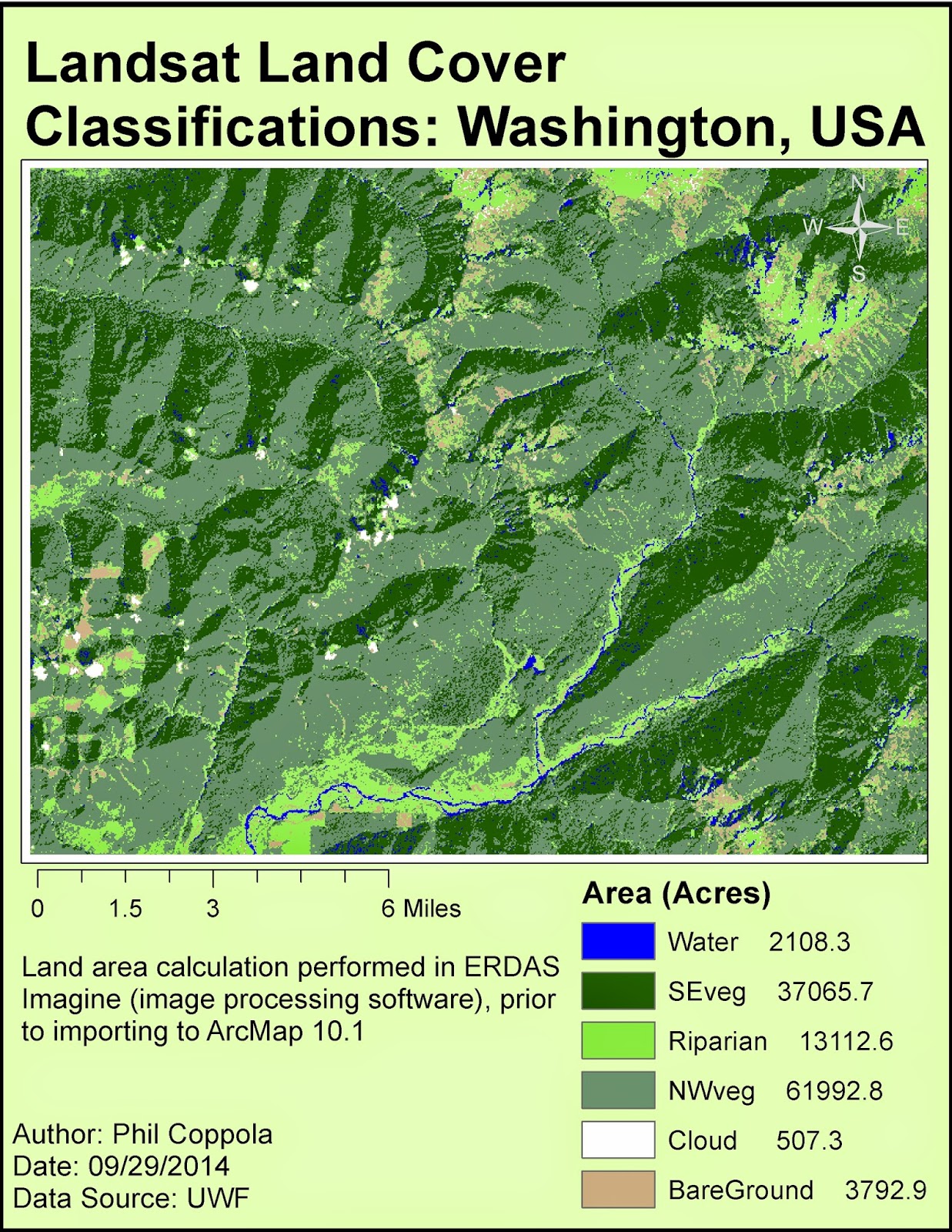
Final map output of landcover generated from
Landsat data first processed in ERDAS Imagine
and ultimately in ArcMap.

This week's lab introduced ERDAS Imagine image analysis software.  This software may be used to aid in the classification of land cover, as well as various other digital image processes and analyses.  We imported land cover raster data sets, manipulated and processed them in Imagine, and ultimately generated a final map output using ArcMap (see map to right).

Lab 4 – Building Networks

This weeks lab involved network analysis.  Routes were determined under a few different conditions including turn restrictions and predicted traffic.  Turn restrictions are relevant when dealing with one-way streets and large road medians.  Predicted traffic influences the time cost of traversing certain roads.  Ultimately, adding model inputs changes the optimal route; however, the significance of the change may be minimal.

Module 4: Ground Truthing and Accuracy Assessment

A map depicting accuracy proofing of LULC data of Pascagoula, MS. 

This lab involved truthing a Land Use Land Cover (LULC) classification map which was generated last week.  Ground truthing was done ex situ using Google StreetView of the area.  Much of the area was inaccessible from StreetView (western marshes) and were truthed using high resolution aerial imagery.

The overall accuracy is determined by comparing random points placed on the original LULC map to those same points found in Google StreetView or aerial imagery.  The overall accuracy of the LULC is determined by the number of "true" points divided by the total points.  The accuracy of my LULC map was 77%.

Lab 3 – Determining Quality of Road Networks

A comparison of "completeness" between the national TIGER data set
and a local, county-level, data set.

This week's assignment involved assessing completeness in road networks.  There are several means to assess the completeness of a road system; however, road length comparisons to known 'accurate' data sets are among the most common.  This involved calculating the total length of road segments within a grid of equal sized squares.

This was applied in lab by assessing the completeness, defined as road length, between a local and national road data set.  The map product at the right shows the comparison.

Lab 3: Land Use / Land Cover Classification Mapping

Above: Map of land cover land use classification of Pascagoula,
Mississippi using USGS LCLU Level II classification scheme.

This week's lab involved creating a land cover land use map of aerial photography using a standardized system.  The aerial photos encompassed portions of Pascagoula, MS and the system was the USGS LCLU system to Level II classification.  The map generated from this process is at right.

Lab 2: Determining Quality of Road Networks

This week's lab involved assessing the accuracy of road networks using a standardized protocol established by the National Standard for Spatial Data Accuracy (NSSDA). We compared the accuracy of two different data sets that represented Albuquerque, NM area.  The first was a local data set from the city of Albuquerque, the second was a national data set from StreetMaps USA (distributed by ESRI).  The process involved extracting intersections from both data sets and then digitizing the "true" location of the intersection using aerial imagery.  The distribution of intersections was quasi-random fairly thorough throughout the study area (see image at right of selected intersections).  It was expect, based on quick initial assessment, that the city data was more accurate than the national data set.  Our results showed this to be true:

Digitized features of the road network database from the city of Albuquerque tested 13.09 feet horizontal accuracy at the 95% confidence level using NSSDA testing procedures.

Digitized features of the road network database from StreetMaps USA tested 688.94 feet horizontal accuracy at the 95% confidence level using NSSDA testing procedures.

Module 2 Lab: Visual Interpretation of Aerial Images

This was my first module for Remote Sensing and Photo Interpretation course.  The focus of this lab was on identifying features within aerial images.  The first exercise involved locating areas of an aerial image that displayed different tones.  Tones, or brightness, may help the user identify features at those locations.  Next, texture, another good diagnostic tool for feature identification was exemplified.

In the second exercise, specific features were identified using size and shape, patterns, associations, and shadows.  Once a single object is positively identified (with a high degree of certainty) than it can be used as a reference in identifying other features.  For example, once you locate and identify a road, you can confirm the identity of a vehicle.  Then a building can be identied.  Because these aerial images have no scale to reference, within-image references are very useful.  A knowledge of the area (Pensacola BEach in map 2 at right) allows the user to determine water and pier features.

Lab 1: Calculating Metrics for Spatial Data Quality

This week was the first lab in Special Topics in GIS.  The focus was on accuracy and precision of data.  Accuracy and Precision are important aspects of all data, including spatial data, and it is important to communicate the accuracy and precision of original data to the receiving audience.

As part of the lab, we were provided an array of waypoints that were collected from a single geographic point using a Garmin GPS device.  We then had to calculate estimates of precision and accuracy after we were then given the "true" reference location.  Below are two outputs of these calculations:

Horizontal Precision (68%): 4.45 meters
Horizontal Accuracy = 3.23 meters

Horizontal precision, which is a metric of the clustering of repeated measurements of a data point, was calculated by determining the average distance of all the repeated measurements to the average of these measurements.  The accuracy was calculated as the difference between the average point from the repeated measurements and a given "true" reference point.