Lab 9 – Accuracy of DEMs

Like any interpolated raster surface, a DEM is derived from an array of measured points, specifically elevations.  What is important for interpolated surfaces is the error introduced during the interpolation process, thus the accuracy and predictive power of the DEM.  The accuracy of a DEM can be determined by comparing interpolated values to known/measured co-located values.  These points can be surveyed after the DEM is created or can be withheld from the interpolation process and used to validate the model.  One method of collected data for DEM generation is via LiDAR.  To check the accuracy of LiDAR-generated DEMs it is important to test several land cover types individually, as they may have different relative inaccuracies.

Module 8 Lab: Thermal & Multispectral Analysis

Multispectral image of Coastal Ecuador highlighting the
color contrast of several distinct features.

The portion of the map that I selected is an agricultural area of the river bank.  I chose this entire area because it was a diverse area, thus providing a good contrast of land features.  There is a freshwater river with a forested island, and on the main land is an agricultural area surrounded by an urban area.  The band combination that was selected appropriately highlights these different features.  Red was linked to Layer 4, Green was linked to Layer 2, and Blue was linked to layer 6 (Thermal IR).  Accordingly, the vegetated island (high NIR, low temp) appear bright red, the urban areas to the east (low NIR, high temp) appear bright blue, and the main river (low NIR, low temp) appears green.

         Further, shape and pattern are useful in identifying these features.  Agricultural lands are often regular polygons (rectangles, or otherwise straight-edged) and would be expected to appear more blue than red in my image, which is the case.  The river and forested island are obvious based on association.

Lab 8 – Surface Interpolation

An output from raster calculator determining the difference between
two output interpolation rasters using the same input points values

This week's lab involved using various interpolation techniques, generating surfaces, and learning limitations of each technique.  Each interpolation process determines the values of unknown cells based on their spatial relationship to known nearby values.  The difference between them is, generally, the weight given to each of the known values - which is usually based on distance and spatial trends.  At right is a comparison of two common interpolation methods: Inverse Distance Weighted interpolation and Spline interpolation.  The most obvious incongruities occurred in areas of low sample density, suggesting these two interpolation techniques duffer in predictions when sample density is low.

Module 7 Lab: Multispectral Analysis

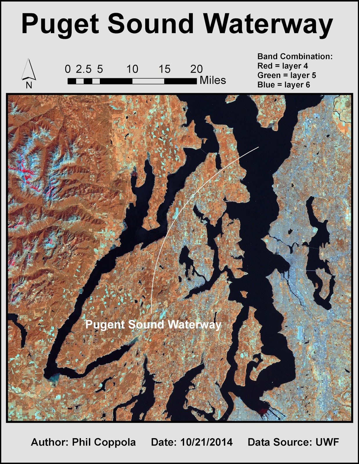 This weeks lab involved using multispectral analyses processes to locate specific features within aerial imagery. Generally four steps are followed: 1) examine histograms of the imagery pixel data; 2) visually examine grey scale image; 3) visually examine multispectral image; 4) use inquire cursor tool to isolate specific cell values. The following are three such examples of this process.  Features are highlighted by their contrast to background features.

Lab 7 – TINs and DEMs

Unmodified TIN

Modified TIN with lake feature burned in

 This week's lav investigated vector-based Triangular Irregular Networks (TINs) and compared them to the raster-based Digital Elevation Models (DEMs).  These are two elevation/topographic models used in GIS to produce accurate representations of real topographical features.  A major diffrence between the two models is that TINs use a series of triangles from several sample points (nodes) of known elevation.  To illustrate how a lake feature can be "burned" into a TIN model, the figures at right depict an original un-modified TIN and the resulting TIN.  Because the TIN uses points of known elevation, the border of the lake feature constitutes a series of points of known elevations.  Thus, the burned-in lake increases the number of triangles, both inside and out of the lake.  The slope inside the lake is 0 throughout.

Module 6 Lab: Spatial Enhancement

Image Enhancement output from ERDAS Imagine and ArcMap
Processing. 

This week's lab involved image enhancement using ERDAS imagine and ArcMap processing tools.  Raw aerial imagery often requires processing steps to produce an image that is spatially and radio-metrically correct.  Image processing software often performs automated enhancement to such images. ERDAS imagine and ArcMap were used to process an image (output seen at right).

Lab 6 – Location-Allocation Modeling

Output of new Market area coverage by distribution facilities

This weeks lab involved using Location Allocation solver in ArcMap.  Location allocation can be used to determine where to place a new store, fire station, or, in the project performed here, service area of a distribution center.  We were provided with an original market area map showing which distribution centers serviced which market areas.  The key is that the original distribution center service areas were generated organically, over-time.  Thus the true nature of our analysis was to determine which service areas should be changed.  The output from the location allocation analysis (see right) shows that several areas (13 total) were better served by a different distribution facility than the one originally selected for it.  Overall,  location allocation solver in ArcMap is a fundamental tool in large-scale data analysis, otherwise not logistically possible.

Lab 5 – Vehicle Routing Problem

This week's lab involved solving a Vehicle Routing Problem (VRP). VRPs are used here to determine optimal routes for fleets of delivery vehicles using a single depot.  Originally, the VRP solver was run with strict route zone restrictions generating an output where several orders were not filled, but profit was maximized.  A second scenario (show at right) was used to allow more flexibility in routing and generated a solution in which all orders were filled.  Customer service is important, thus the second scenario is the more desirable one.