Participation Assignment #2: Migration Patterns of Northern Saw-Whet Owls

 Beckett, Sean R. and Glen A. Proudfoot. 2011. Large-scale Movement and Migration of Northen Saw-Whet Owls in Eastern North America.  The Wilson Journal of Ornithology 123(3):521-535.

In this paper, researchers mine a bird banding database to tease apart patterns of migration and large scale movement for the Northern Saw-whet Owl (NSWO) in eastern North America.  The United States Geological Survey (USGS) oversees several bird banding stations in the United States and manages the large database produced from them.  Bird banding stations are permanent, semi-permanent, or temporary field locations where ornithologists capture target bird species and place on them leg bands engraved with unique serial numbers.  The overall number of birds caught at specific banding stations may fluctuate seasonally or annually; thus, population trends or mass movement patterns may be detected using relevant spatiotemporal analyses.  Further, birds with bands can be recaptured within or between years so that individual movement and migration routes can be analyzed.

The Northern Saw-Whet Owl is a small owl that resides in the United States.  This study attempts to use banding records of this bird to determine if it migrates southward during the fall season, if individuals follow similar migration routes between years, and whether there is any age-related differences in movement.  They use a GIS (ArcView 9.3; ESRI 2008) to complete these analyses.

They examine the number of banded NSWOs using of 01° latitudinal lines as groups.  They find that the peak banding day – i.e. the mean Julian day – occurs later in the year as your move further south.  Thus they determined that NSWOs have a mass migration south during the fall months (fig. 3, Beckett & Proudfoot 2011).  Then, by creating vectors from original owl capture to recapture locations, they generated a rose diagram depicting the southerly movement for the birds during fall (fig. 5, Beckett & Proudfoot 2011).

This paper is significant in that it answers a large-scale question utilizing a public-access database – in other words the data was gathered, not collect, by the researchers.  They illustrate the use of databases and GISs as a foundational tool for understanding ecology of animal populations.  With increasing technological advances and utilization, similar research will continue to be produced.

link to paper: http://www.projectowlnet.org/wp-content/uploads/2011/09/Beckett-and-Proudfoot-2011-Wilson.pdf

Module 9: Debugging & Error Handling

Output for Script 1

Output for Script 2

Output for Script 3

This weeks lab involved debugging and error handling, perhaps the most frustrating part of writing scripts in Python.  There are three types of errors encounter in Python: syntax errors, exceptions, and logic errors.  They can arise from improper character entry into the program, or from errors in geoprocessing.

The assignment involved debugging three scripts in various ways, creating the outputs seen at right.  PythonWin contains its own debugging interface, which was used to help the user locate or trap exceptions.  In the Output for Script 3 (below), an error message is presented, but the script was allowed to continue. Essentially, that portion/block of script was passed over.

Module 8: Working with Rasters

Final raster output that meets all criteria.

This week's lab involved working with rasters using the spatial analyst module in arcpy package.  Rasters allow for the display of continuous spatial phenomena and analysis using a GIS has made complex processes relatively simple.  The final lab output was a raster meeting three specific criteria.  These were: a specific landcover type, a slope between 5 - 20 degrees, and an aspect between 150 - 270 degrees.  The script written uses only DEM and landcover inputs.  At rights is a final raster output, below is a discussion of an issue that I encountered during the lab and how it was resolved.

1.     The only issue I had was that my final map displayed a raster with values of 1, 0, and NoData and thus looked different than the example shown on the assignment PDF.  Immediately I recognized that this was likely due to the landcover reclassification step.  The original script was as follows:

>>> outreclass = Reclassify("landcover", "VALUE", myremap, “NoData”)

2.       I investigated the Reclassify tool’s syntax through ArcMap help > Reclassify tool.

3.       “NoData” was displaying differently because I had specified it to do so in the script.  The final argument of how to represent NoData was optional, but I had entered it in.  The original script was copied from the Mod8 Exercise, this was the root of the problem.  In the Mod8 Exercise we purposely wanted to specify cells with NoData; however, in the Mod8 Assignment, we want to specify all cells that do not meet the criteria with a value of 0.

4.       Therefore, I removed the last, optional argument in the original script, creating the following final script, which ultimately produced the correct final raster:

>>> outreclass = Reclassify("landcover", "VALUE", myremap)

Week 9: Corridor Analysis

Corridor model

This week's assignment involved creating cost paths and corridors.  Ultimately, a model for black bear movement between two national park units was created.  Cost paths and corridors are used to predict the pathways that are least costly to construct (in the case of roads and utilities, etc.) or traverse (in the case of wildlife, utilities, etc).

The corridor output at right shows a predicted black bear corridor.  The parameters used to create this corridor were elevation, land use (not shown), and roads (not shown).  Bears prefer certain elevations, certain habitats, and avoid roads.  So a suitability analysis was performed to find the most bear-friendly areas.  Then the corridor analysis was use to create the best path between the two units.

Module 7: Working with Geometries

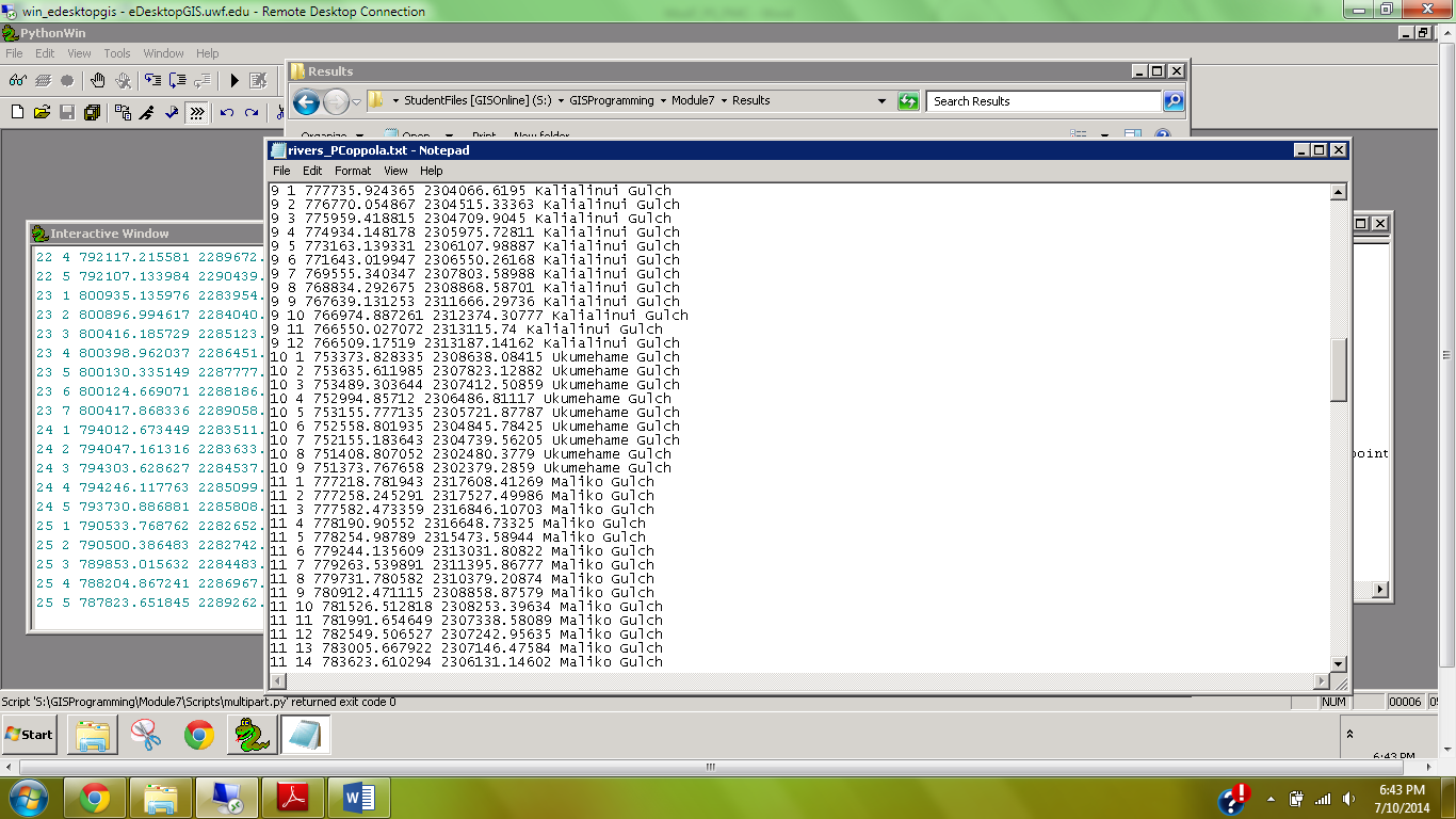
Screenshot of rivers_PCoppola.txt file

This week's lab focused on the conceptual and tangible connection between geometric/vector objects and the attribute table.  Specifically, we worked with features, arrays, and vertices by using cursors and tokens to produce a .txt file of select items from the attribute table (see screenshot at right).  The feature was a system of rivers (polyline feature class) on Hawaii.  We wrote a script that would iterate through all the arrays of this feature class and provide an output of the feature number, vertex number, x,y-coordinates, and feature name.  This required nested for loops to iterate over the embedded arrays.

Week 8: Network Analysis

This week's assignment dealt with network analysis.  At right is a service area analysis depicting the change of catchment coverage for Austin Community College after the closure of the Cypress Creek Campus.  The service area consists of several layered areas within a specified range.  It is clear that coverage changes, and the ultimate effect of this change was further assessed using demographic data.  For example, over 1,000 college student aged citizens who were closest the the closing campus must now attend a different campus, thus increasing the student-averaged travel time to any campus.