Lab 15 – Dasymetric Mapping

Dasymetric mapping is a mapping technique that involves using ancillary spatial data to improve the visualization and accuracy of spatial phenomenon that is known to not be uniformly distributed throughout the landscape.  An example of this is population density, which is presumed to vary greatly spatially within the census tracts which are used to estimate density.  By using smaller aerial units, say census blocks, we know that the population density is not uniform within the census tract.  By using land cover data, the accuracy can be improved further, as we presume that population density is zero in forest areas and water bodies otherwise not accounted for.

In this lab we were given census tract data and high school boundary data and told to determine the approximate number of students who fall in each school zone.  The issue is that the census tract polygons and the school boundaries do not align in any useful way.  By splitting census tracts that fell within different high school boundaries, then weighting the population estimate based on the area that fell in each boundary (i.e. aerial weighting), a relatively accurate and easy-to-produce estimate was determined; error was at 10.95%.  Then, by incorporating land cover data, specifically imperviousness, the error decreased to 10.19%.  The imperviousness of each split census tract was used to weight the proportion of the entire census tract that would be assigned to it.  Using the dasymtric mapping method was useful for projects like this, because surveying a community individually would require large amounts of time and resources, though accuracy would be higher.

Lab 14 – Spatial Data Aggregation

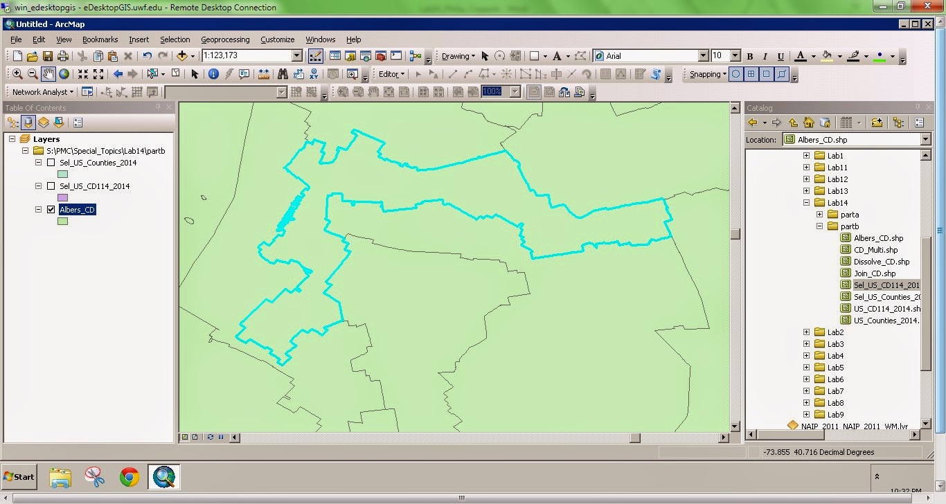
Gerrymandering is the manipulation of political boundaries so as to favor one party or class.  The favorable outcome is a result of the statistical influence of scale and zonation of areal units.  This manipulation of boundaries often produces odd shaped districts.  The two images to the right show two outcomes of gerrymandering.  The top image depicts a district boundary that chops up a county.  The bottom image depicts a very elongated, irregular district.